import os
import random
import numpy as np
import pandas as pd
from sklearn.metrics import mean_squared_error
from sklearn.model_selection import train_test_split
from sklearn.preprocessing import MinMaxScaler
import plotly.express as px
import plotly.graph_objs as go
from plotly.offline import init_notebook_mode
import requests
# %load_ext autoreload
# %autoreload 2
from pytorch_tabular import TabularModel
from pytorch_tabular.models import (
    CategoryEmbeddingModelConfig,
    GatedAdditiveTreeEnsembleConfig,
    MDNConfig
)
from pytorch_tabular.config import (
    DataConfig,
    OptimizerConfig,
    TrainerConfig,
    ExperimentConfig,
)
# from pytorch_tabular.categorical_encoders import CategoricalEmbeddingTransformer
from pytorch_tabular.models.common.heads import LinearHeadConfig, MixtureDensityHeadConfig
np.random.seed(42)
Utility Functions
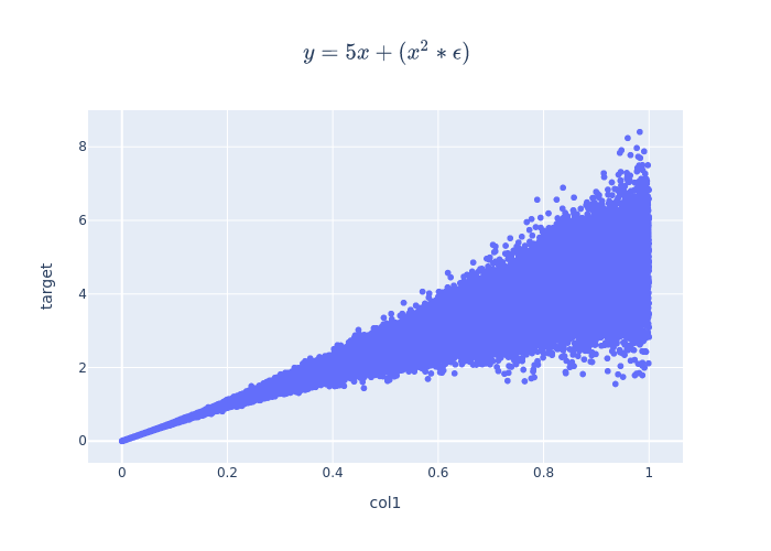
def generate_linear_example(samples=int(1e5)):
x_data = np.random.sample(samples)[:, np.newaxis].astype(np.float32)
y_data = np.add(5*x_data, np.multiply((x_data)**2, np.random.standard_normal(x_data.shape)))
x_train, x_valid, y_train, y_valid = train_test_split(x_data, y_data, test_size=0.5, random_state=42)
x_test = np.linspace(0.,1.,int(1e3))[:, np.newaxis].astype(np.float32)
df_train = pd.DataFrame({"col1": x_train.ravel(), "target": y_train.ravel()})
df_valid = pd.DataFrame({"col1": x_valid.ravel(), "target": y_valid.ravel()})
# test = sorted(df_valid.col1.round(3).unique())
# df_test = pd.DataFrame({"col1": test})
df_test = pd.DataFrame({"col1": x_test.ravel()})
return (df_train, df_valid, df_test, ["target"])
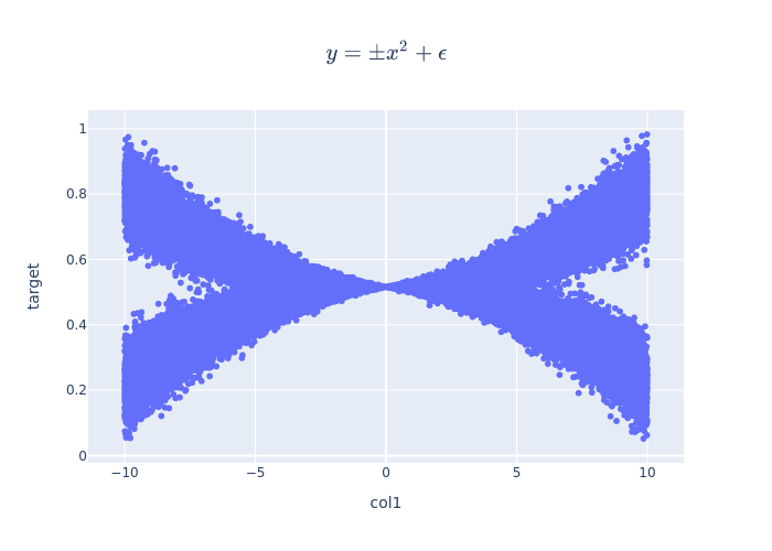
def generate_non_linear_example(samples=int(1e5)):
x_data = np.float32(np.random.uniform(-10, 10, (1, samples)))
r_data = np.array([np.random.normal(scale=np.abs(i)) for i in x_data])
y_data = np.float32(np.square(x_data)+r_data*2.0)
x_data2 = np.float32(np.random.uniform(-10, 10, (1, samples)))
r_data2 = np.array([np.random.normal(scale=np.abs(i)) for i in x_data2])
y_data2 = np.float32(-np.square(x_data2)+r_data2*2.0)
x_data = np.concatenate((x_data,x_data2),axis=1).T
y_data = np.concatenate((y_data,y_data2),axis=1).T
min_max_scaler = MinMaxScaler()
y_data = min_max_scaler.fit_transform(y_data)
x_train, x_valid, y_train, y_valid = train_test_split(x_data, y_data, test_size=0.5, random_state=42, shuffle=True)
x_test = np.linspace(-10,10,int(1e3))[:, np.newaxis].astype(np.float32)
df_train = pd.DataFrame({"col1": x_train.ravel(), "target": y_train.ravel()})
df_valid = pd.DataFrame({"col1": x_valid.ravel(), "target": y_valid.ravel()})
# test = sorted(df_valid.col1.round(3).unique())
# df_test = pd.DataFrame({"col1": test})
df_test = pd.DataFrame({"col1": x_test.ravel()})
return (df_train, df_valid, df_test, ["target"])
def generate_step_linear_example(samples=int(1e5)):
x_data = np.random.sample(samples)[:, np.newaxis].astype(np.float32)
y_data = np.zeros(x_data.shape)
mask = x_data<0.5
y_data[mask] = np.add(5*x_data[mask], np.multiply((x_data[mask])**2, np.random.standard_normal(x_data[mask].shape)))
y_data[~mask] = np.add(100*x_data[~mask]+x_data[~mask]**2 , np.multiply((x_data[~mask])**2, np.random.standard_normal(x_data[~mask].shape)))
min_max_scaler = MinMaxScaler()
y_data = min_max_scaler.fit_transform(y_data)
x_train, x_valid, y_train, y_valid = train_test_split(x_data, y_data, test_size=0.5, random_state=42, shuffle=True)
x_test = np.linspace(0.,1.,int(1e3))[:, np.newaxis].astype(np.float32)
df_train = pd.DataFrame({"col1": x_train.ravel(), "target": y_train.ravel()})
df_valid = pd.DataFrame({"col1": x_valid.ravel(), "target": y_valid.ravel()})
# test = sorted(df_valid.col1.round(3).unique())
# df_test = pd.DataFrame({"col1": test})
df_test = pd.DataFrame({"col1": x_test.ravel()})
return (df_train, df_valid, df_test, ["target"])
def generate_gaussian_mixture(samples=int(1e5)):
x_data = np.random.sample(samples)[:, np.newaxis].astype(np.float32)
pi = np.sin(x_data)+3*x_data*np.cos(x_data)
pi = pi/pi.max()
# g1 = np.random.sample(samples)*4*x_data.squeeze()
# g2 = np.random.sample(samples)*15*x_data.squeeze()
g1 = 2*x_data.squeeze() + 0.5*np.random.sample(samples)
g2 = 8*x_data.squeeze() + 0.5*np.random.sample(samples)
y_data = pi.round().squeeze()*g1 + (1-pi.round().squeeze())*g2
y_data = y_data.reshape(-1,1)
x_train, x_valid, y_train, y_valid = train_test_split(x_data, y_data, test_size=0.5, random_state=42)
x_test = np.linspace(0.,1.,int(1e3))[:, np.newaxis].astype(np.float32)
df_train = pd.DataFrame({"col1": x_train.ravel(), "target": y_train.ravel()})
df_valid = pd.DataFrame({"col1": x_valid.ravel(), "target": y_valid.ravel()})
# test = sorted(df_valid.col1.round(3).unique())
# df_test = pd.DataFrame({"col1": test})
df_test = pd.DataFrame({"col1": x_test.ravel()})
return (df_train, df_valid, df_test, ["target"])
def latex_to_png( formula, file):
tfile = file
r = requests.get( 'http://latex.codecogs.com/png.latex?\dpi{300} \huge %s' % formula )
with open( tfile, 'wb' ) as f:
# f = open( tfile, 'wb' )
f.write( r.content )
# f.close()
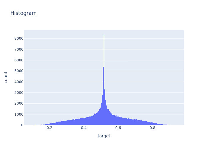
Linear Example
Plot
# display(Math(r"$y = 5x + (x^2 * \epsilon)$"+"\n"+r"$\epsilon \backsim \mathcal{N}(0,1)$"))
fig = px.scatter(df_train, x="col1", y="target", title=r"$y = 5x + (x^2 * \epsilon)$"+"\n"+r"$\epsilon \backsim \mathcal{N}(0,1)$")
fig.update_layout(
    title={
        'y':0.9,
        'x':0.5,
        'xanchor': 'center',
        'yanchor': 'top'})
fig.write_image("imgs/prob_reg_fig_1.png")
Training the MDN
Define the Configs
epochs = 15
batch_size = 128
steps_per_epoch = int((len(df_train)//batch_size)*0.9)
data_config = DataConfig(
    target=['target'],
    continuous_cols=['col1'],
    categorical_cols=[],
#         continuous_feature_transform="quantile_uniform"
)
trainer_config = TrainerConfig(
    auto_lr_find=True, # Runs the LRFinder to automatically derive a learning rate
    batch_size=batch_size,
    max_epochs=epochs,
    early_stopping="valid_loss",
    early_stopping_patience=5,
    checkpoints="valid_loss"
)

optimizer_config = OptimizerConfig(lr_scheduler="ReduceLROnPlateau", lr_scheduler_params={"patience":3})

mdn_head_config = MixtureDensityHeadConfig(num_gaussian=1).__dict__

backbone_config_class = "CategoryEmbeddingModelConfig"
backbone_config = dict(
    task="backbone",
    layers="128-64",  # Number of nodes in each layer
    activation="ReLU",  # Activation between each layers
    initialization="kaiming"
)

model_config = MDNConfig(
    task="regression",
    backbone_config_class=backbone_config_class,
    backbone_config_params=backbone_config,
    head_config=mdn_head_config,
    learning_rate=1e-3,
)
tabular_model = TabularModel(
    data_config=data_config,
    model_config=model_config,
    optimizer_config=optimizer_config,
    trainer_config=trainer_config
)
Training the Model
Predictions and Visualization
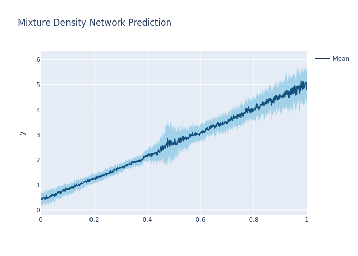
fig = go.Figure([
    go.Scatter(
        name='Mean',
        x=pred_df['col1'],
        y=pred_df['target_prediction'],
        mode='lines',
        line=dict(color='rgba(28,53,94,1)'),
    ),
    go.Scatter(
        name='Upper Bound',
        x=pred_df['col1'],
        y=pred_df['target_q75'],
        mode='lines',
        marker=dict(color='rgba(0,147,201,0.3)'),
        line=dict(width=0),
        showlegend=False
    ),
    go.Scatter(
        name='Lower Bound',
        x=pred_df['col1'],
        y=pred_df['target_q25'],
        marker=dict(color="#444"),
        line=dict(width=0),
        mode='lines',
        fillcolor='rgba(0,147,201,0.3)',
        fill='tonexty',
        showlegend=False
    )
])
fig.update_layout(
    yaxis_title='y',
    title='Mixture Density Network Prediction',
    hovermode="x"
)
# fig.show()
fig.write_image("imgs/prob_reg_mdn_1.png")
Non-Linear Example
Plot
Training a FeedForward
Define the Configs
epochs = 200
batch_size = 2048
steps_per_epoch = int((len(df_train)//batch_size)*0.9)
data_config = DataConfig(
    target=['target'],
    continuous_cols=['col1'],
    categorical_cols=[],
#         continuous_feature_transform="quantile_uniform"
)
trainer_config = TrainerConfig(
    auto_lr_find=True, # Runs the LRFinder to automatically derive a learning rate
    batch_size=batch_size,
    max_epochs=epochs,
    early_stopping="valid_loss",
    early_stopping_patience=5,
    checkpoints="valid_loss"
)
optimizer_config = OptimizerConfig(lr_scheduler="ReduceLROnPlateau", lr_scheduler_params={"patience":3})
model_config = CategoryEmbeddingModelConfig(
    task="regression",
    layers="16-8",  # Number of nodes in each layer
    activation="ReLU",  # Activation between each layers
    head="LinearHead",
    learning_rate=1e-3,
)
tabular_model = TabularModel(
    data_config=data_config,
    model_config=model_config,
    optimizer_config=optimizer_config,
    trainer_config=trainer_config
)
Training the Model
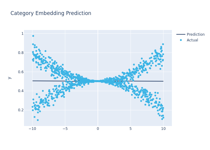
Predictions and Visualization
fig = go.Figure([
    go.Scatter(
        name='Prediction',
        x=pred_df['col1'],
        y=pred_df['target_prediction'],
        mode='lines',
        line=dict(color='rgba(28,53,94,1)'),
    ),
    go.Scatter(
        name='Actual',
        x=pred_df['col1'],
        y=pred_df['target'],
        mode='markers',
        line=dict(color='rgba(60,180,229,1)'),
    ),
])
fig.update_layout(
    yaxis_title='y',
    title='Category Embedding Prediction',
    hovermode="x"
)
# fig.show()
fig.write_image("imgs/prob_reg_non_mdn_2.png")
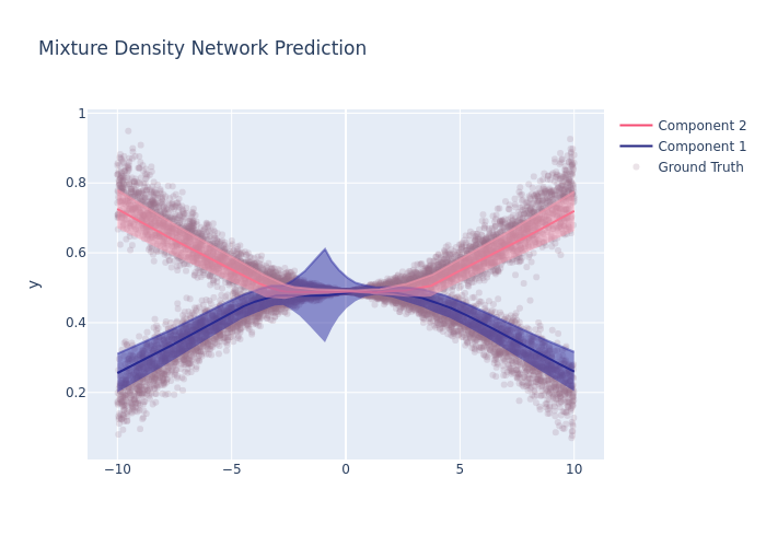
Training the MDN
Define the Configs
epochs = 200
batch_size = 2048
steps_per_epoch = int((len(df_train)//batch_size)*0.9)
data_config = DataConfig(
    target=['target'],
    continuous_cols=['col1'],
    categorical_cols=[],
#         continuous_feature_transform="quantile_uniform"
)
trainer_config = TrainerConfig(
    auto_lr_find=False, # Runs the LRFinder to automatically derive a learning rate
    batch_size=batch_size,
    max_epochs=epochs,
    early_stopping="valid_loss",
    early_stopping_patience=5,
    checkpoints="valid_loss"
)
optimizer_config = OptimizerConfig(lr_scheduler="ReduceLROnPlateau", lr_scheduler_params={"patience":3})

mdn_head_config = MixtureDensityHeadConfig(num_gaussian=2, weight_regularization=2, lambda_mu=10, lambda_pi=5).__dict__

backbone_config_class = "CategoryEmbeddingModelConfig"
backbone_config = dict(
    task="backbone",
    layers="128-64",  # Number of nodes in each layer
    activation="ReLU",  # Activation between each layers
    head=None,
)

model_config = MDNConfig(
    task="regression",
    backbone_config_class=backbone_config_class,
    backbone_config_params=backbone_config,
    head_config=mdn_head_config,
    learning_rate=1e-3,
)

tabular_model = TabularModel(
    data_config=data_config,
    model_config=model_config,
    optimizer_config=optimizer_config,
    trainer_config=trainer_config
)
Training the Model
Predictions and Visualization
fig = go.Figure([
    go.Scatter(
        name='Ground Truth',
        x=df['col1'],
        y=df['target'],
        mode='markers',
        line=dict(color='rgba(153, 115, 142, 0.2)'),
    ),
    go.Scatter(
        name='Component 1',
        x=pred_df['col1'],
        y=pred_df['mu_0'],
        mode='lines',
        line=dict(color='rgba(36, 37, 130, 1)'),
    ),
    go.Scatter(
        name='Component 2',
        x=pred_df['col1'],
        y=pred_df['mu_1'],
        mode='lines',
        line=dict(color='rgba(246, 76, 114, 1)'),
    ),
    go.Scatter(
        name='Upper Bound 1',
        x=pred_df['col1'],
        y=pred_df['mu_0']+pred_df['sigma_0'],
        mode='lines',
        marker=dict(color='rgba(47, 47, 162, 0.5)'),
#         line=dict(width=0),
        showlegend=False
    ),
    go.Scatter(
        name='Lower Bound 1',
        x=pred_df['col1'],
        y=pred_df['mu_0']-pred_df['sigma_0'],
        marker=dict(color="#444"),
        line=dict(width=0),
        mode='lines',
        fillcolor='rgba(47, 47, 162, 0.5)',
        fill='tonexty',
        showlegend=False
    ),
    go.Scatter(
        name='Upper Bound 2',
        x=pred_df['col1'],
        y=pred_df['mu_1']+pred_df['sigma_1'],
        mode='lines',
        marker=dict(color='rgba(250, 152, 174, 0.5)'),
#         line=dict(width=0),
        showlegend=False
    ),
    go.Scatter(
        name='Lower Bound 2',
        x=pred_df['col1'],
        y=pred_df['mu_1']-pred_df['sigma_1'],
        marker=dict(color="#444"),
        line=dict(width=0),
        mode='lines',
        fillcolor='rgba(250, 152, 174, 0.5)',
        fill='tonexty',
        showlegend=False
    ),
])
fig.update_layout(
    yaxis_title='y',
    title='Mixture Density Network Prediction',
    hovermode="x"
)
# fig.show()
fig.write_image("imgs/prob_reg_mdn_2.png")
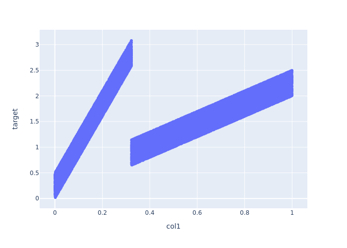
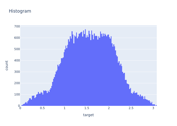
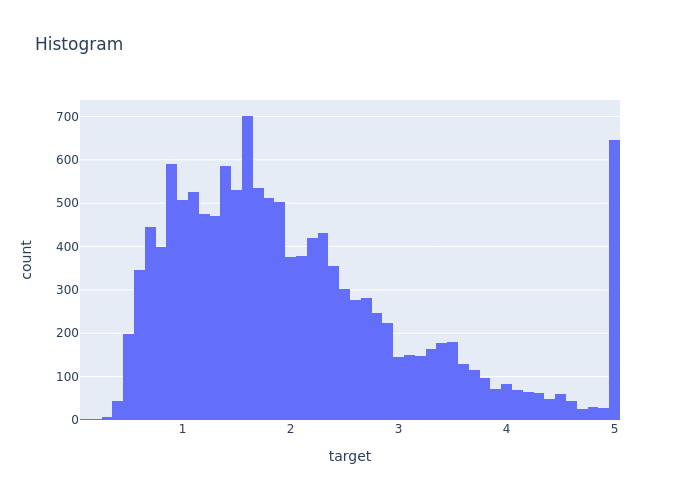
Gaussian Mixture
Plot
eqn = r'$\pi = \frac{sin(x) + 3xcos(x)}{max \left (sin(x) + 3xcos(x) \right )} \\ \\ g1 = 2x + 0.5 \epsilon \rightarrow  \epsilon \backsim \mathcal{N}(0,1) \\ g2 = 8x + 0.5 \epsilon \rightarrow  \epsilon \backsim \mathcal{N}(0,1) \\ p = Bernoulli(pi) \rightarrow \text{Samples one of two outcomes based on the value of } \pi \\ y = p \times g1 + (1-p) \times g2$'
display(Math(eqn))
fig = px.scatter(df_train, x="col1", y="target")
fig.update_layout(
    title={
        'y':0.9,
        'x':0.5,
        'xanchor': 'center',
        'yanchor': 'top'})
fig.write_image("imgs/prob_reg_fig_3.png")
Training a FeedForward
Define the Configs
epochs = 200
batch_size = 2048
steps_per_epoch = int((len(df_train)//batch_size)*0.9)
data_config = DataConfig(
    target=['target'],
    continuous_cols=['col1'],
    categorical_cols=[],
#         continuous_feature_transform="quantile_uniform"
)
trainer_config = TrainerConfig(
    auto_lr_find=True, # Runs the LRFinder to automatically derive a learning rate
    batch_size=batch_size,
    max_epochs=epochs,
    early_stopping="valid_loss",
    early_stopping_patience=5,
    checkpoints="valid_loss"
)

optimizer_config = OptimizerConfig(lr_scheduler="ReduceLROnPlateau", lr_scheduler_params={"patience":3})

model_config = CategoryEmbeddingModelConfig(
    task="regression",
    layers="16-8",  # Number of nodes in each layer
    activation="ReLU",  # Activation between each layers
    head="LinearHead",
    learning_rate=1e-3,
)

tabular_model = TabularModel(
    data_config=data_config,
    model_config=model_config,
    optimizer_config=optimizer_config,
    trainer_config=trainer_config
)
Training the Model
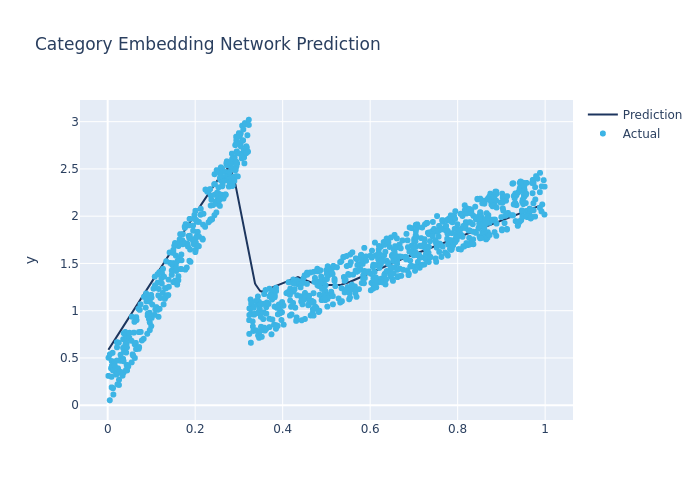
Predictions and Visualization
fig = go.Figure([
    go.Scatter(
        name='Prediction',
        x=pred_df['col1'],
        y=pred_df['target_prediction'],
        mode='lines',
        line=dict(color='rgba(28,53,94,1)'),
    ),
    go.Scatter(
        name='Actual',
        x=pred_df['col1'],
        y=pred_df['target'],
        mode='markers',
        line=dict(color='rgba(60,180,229,1)'),
    ),
])
fig.update_layout(
    yaxis_title='y',
    title='Category Embedding Network Prediction',
    hovermode="x"
)
fig.write_image("imgs/prob_reg_non_mdn_3.png")
Training the MDN
Define the Configs
epochs = 200
batch_size = 2048
steps_per_epoch = int((len(df_train)//batch_size)*0.9)
data_config = DataConfig(
    target=['target'],
    continuous_cols=['col1'],
    categorical_cols=[],
#         continuous_feature_transform="quantile_uniform"
)
trainer_config = TrainerConfig(
    auto_lr_find=True, # Runs the LRFinder to automatically derive a learning rate
    batch_size=batch_size,
    max_epochs=epochs,
    early_stopping_patience = 5,
    early_stopping="valid_loss",
    checkpoints="valid_loss",
    load_best=True
)

optimizer_config = OptimizerConfig(lr_scheduler="ReduceLROnPlateau", lr_scheduler_params={"patience":3})

mdn_head_config = MixtureDensityHeadConfig(num_gaussian=2, weight_regularization=2).__dict__

backbone_config_class = "CategoryEmbeddingModelConfig"
backbone_config = dict(
    task="backbone",
    layers="128-64",  # Number of nodes in each layer
    activation="ReLU",  # Activation between each layers
    head=None,
)

model_config = MDNConfig(
    task="regression",
    backbone_config_class=backbone_config_class,
    backbone_config_params=backbone_config,
    head_config=mdn_head_config,
    learning_rate=1e-3,
)

tabular_model = TabularModel(
    data_config=data_config,
    model_config=model_config,
    optimizer_config=optimizer_config,
    trainer_config=trainer_config
)
Training the Model
Predictions and Visualization
fig = go.Figure([
    go.Scatter(
        name='Ground Truth',
        x=df['col1'],
        y=df['target'],
        mode='markers',
        line=dict(color='rgba(153, 115, 142, 0.2)'),
    ),
    go.Scatter(
        name='Component 1',
        x=pred_df['col1'],
        y=pred_df['mu_0'],
        mode='lines',
        line=dict(color='rgba(90, 92, 237, 1)'),
    ),
    go.Scatter(
        name='Component 2',
        x=pred_df['col1'],
        y=pred_df['mu_1'],
        mode='lines',
        line=dict(color='rgba(246, 76, 114, 1)'),
    ),
    go.Scatter(
        name='Upper Bound 1',
        x=pred_df['col1'],
        y=pred_df['mu_0']+pred_df['sigma_0'],
        mode='lines',
        marker=dict(color='rgba(47, 47, 162, 0.5)'),
#         line=dict(width=0),
        showlegend=False
    ),
    go.Scatter(
        name='Lower Bound 1',
        x=pred_df['col1'],
        y=pred_df['mu_0']-pred_df['sigma_0'],
        marker=dict(color="#444"),
        line=dict(width=0),
        mode='lines',
        fillcolor='rgba(47, 47, 162, 0.5)',
        fill='tonexty',
        showlegend=False
    ),
    go.Scatter(
        name='Upper Bound 2',
        x=pred_df['col1'],
        y=pred_df['mu_1']+pred_df['sigma_1'],
        mode='lines',
        marker=dict(color='rgba(250, 152, 174, 0.5)'),
#         line=dict(width=0),
        showlegend=False
    ),
    go.Scatter(
        name='Lower Bound 2',
        x=pred_df['col1'],
        y=pred_df['mu_1']-pred_df['sigma_1'],
        marker=dict(color="#444"),
        line=dict(width=0),
        mode='lines',
        fillcolor='rgba(250, 152, 174, 0.5)',
        fill='tonexty',
        showlegend=False
    ),
])
fig.update_layout(
    yaxis_title='y',
#     yaxis_range=[0,1],
    title='Mixture Density Network Prediction',
    hovermode="x",
    yaxis_range=[df['target'].min()*0.85, df['target'].max()*1.15]
)
fig.write_image("imgs/prob_reg_mdn_3.png")
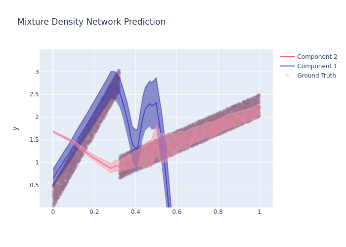
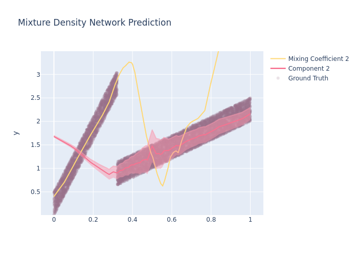
fig = go.Figure([
go.Scatter(
name='Ground Truth',
x=df['col1'],
y=df['target'],
mode='markers',
line=dict(color='rgba(153, 115, 142, 0.2)'),
),
go.Scatter(
name='Component 1',
x=pred_df['col1'],
y=pred_df['mu_0'],
mode='lines',
line=dict(color='rgba(90, 92, 237, 1)'),
),
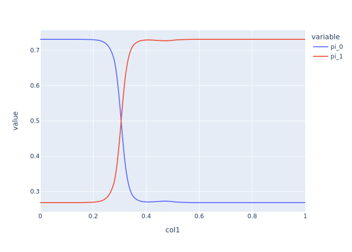
go.Scatter(
name='Mixing Coefficient 1',
x=pred_df['col1'],
y=pred_df['pi_1'],
mode='lines',
line=dict(color='rgba(255, 216, 117, 1)'),
),
go.Scatter(
name='Upper Bound 1',
x=pred_df['col1'],
y=pred_df['mu_0']+pred_df['sigma_0'],
mode='lines',
marker=dict(color='rgba(47, 47, 162, 0.5)'),
# line=dict(width=0),
showlegend=False
),
go.Scatter(
name='Lower Bound 1',
x=pred_df['col1'],
y=pred_df['mu_0']-pred_df['sigma_0'],
marker=dict(color="#444"),
line=dict(width=0),
mode='lines',
fillcolor='rgba(47, 47, 162, 0.5)',
fill='tonexty',
showlegend=False
),
])
fig.update_layout(
yaxis_title='y',
# yaxis_range=[-0.2,1],
title='Mixture Density Network Prediction',
hovermode="x",
yaxis_range=[df['target'].min()*0.85, df['target'].max()*1.15]
)
fig.write_image("imgs/prob_reg_mixing1_3.png")
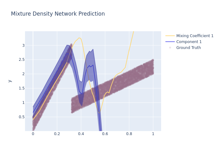
fig = go.Figure([
    go.Scatter(
        name='Ground Truth',
        x=df['col1'],
        y=df['target'],
        mode='markers',
        line=dict(color='rgba(153, 115, 142, 0.2)'),
    ),

    go.Scatter(
        name='Component 2',
        x=pred_df['col1'],
        y=pred_df['mu_1'],
        mode='lines',
        line=dict(color='rgba(246, 76, 114, 1)'),
    ),

    go.Scatter(
        name='Mixing Coefficient 2',
        x=pred_df['col1'],
        y=pred_df['pi_1'],
        mode='lines',
        line=dict(color='rgba(255, 216, 117, 1)'),
    ),

    go.Scatter(
        name='Upper Bound 2',
        x=pred_df['col1'],
        y=pred_df['mu_1']+pred_df['sigma_1'],
        mode='lines',
        marker=dict(color='rgba(250, 152, 174, 0.5)'),
#         line=dict(width=0),
        showlegend=False
    ),
    go.Scatter(
        name='Lower Bound 2',
        x=pred_df['col1'],
        y=pred_df['mu_1']-pred_df['sigma_1'],
        marker=dict(color="#444"),
        line=dict(width=0),
        mode='lines',
        fillcolor='rgba(250, 152, 174, 0.5)',
        fill='tonexty',
        showlegend=False
    ),
])
fig.update_layout(
    yaxis_title='y',
#     yaxis_range=[-0.2,1],
    title='Mixture Density Network Prediction',
    hovermode="x",
    yaxis_range=[df['target'].min()*0.85, df['target'].max()*1.15]
)
fig.write_image("imgs/prob_reg_mixing2_3.png")
Boston Housing Dataset
from sklearn.datasets import fetch_california_housing
target_col = "target"
data = fetch_california_housing(return_X_y=False)
X = pd.DataFrame(data['data'], columns=data['feature_names'])
cont_cols = X.columns.tolist()
cat_cols = []
y = data['target']
X[target_col] = y
df_train, df_test = train_test_split(X, test_size=0.2, random_state=42)
df_train, df_valid = train_test_split(df_train, test_size=0.2, random_state=42)
Plot
Training the MDN
Define the Configs
Let's use a nifty util function in the package to figure out the centers of the possible gaussian components. It internally runs a Kmeans and returns the cluster centroids and lets set that as the bias initialization
epochs = 1000
batch_size = 2048
steps_per_epoch = int((len(df_train)//batch_size)*0.9)
data_config = DataConfig(
    target=['target'],
    continuous_cols=cont_cols,
    categorical_cols=cat_cols,
#         continuous_feature_transform="quantile_uniform"
)
trainer_config = TrainerConfig(
    auto_lr_find=True, # Runs the LRFinder to automatically derive a learning rate
    batch_size=batch_size,
    max_epochs=epochs,
    early_stopping="valid_loss",
    early_stopping_patience=5,
    checkpoints="valid_loss",
    load_best=True
)

optimizer_config = OptimizerConfig(lr_scheduler="ReduceLROnPlateau", lr_scheduler_params={"patience":3})

mdn_head_config = MixtureDensityHeadConfig(
    num_gaussian=4,
    weight_regularization=2,
    mu_bias_init=mu_init
).__dict__

#lambda_pi=10,
#lambda_sigma=1,

backbone_config_class = "CategoryEmbeddingModelConfig"
backbone_config = dict(
    task="backbone",
    layers="200-100",  # Number of nodes in each layer
    activation="ReLU",  # Activation between each layers
    head=None,
)

model_config = MDNConfig(
    task="regression",
    backbone_config_class=backbone_config_class,
    backbone_config_params=backbone_config,
    head_config=mdn_head_config,
    learning_rate=1e-3,
)


tabular_model = TabularModel(
    data_config=data_config,
    model_config=model_config,
    optimizer_config=optimizer_config,
    trainer_config=trainer_config
)
Training the Model
Predictions and Visualization
import scipy.stats as ss

def plot_normal(x_range, mu=0, sigma=1, cdf=False, **kwargs):
    '''
    Plots the normal distribution function for a given x range
    If mu and sigma are not provided, standard normal is plotted
    If cdf=True cumulative distribution is plotted
    Passes any keyword arguments to matplotlib plot function
    '''
    x = x_range
    if cdf:
        y = ss.norm.cdf(x, mu, sigma)
    else:
        y = ss.norm.pdf(x, mu, sigma)
    return x,y
def get_pdf(idx):
    row = pred_df.iloc[idx]
    pi = torch.from_numpy(row[['pi_0','pi_1','pi_2','pi_3']].values).unsqueeze(0)
    mu = torch.from_numpy(row[['mu_0','mu_1','mu_2','mu_3']].values).unsqueeze(0)
    sigma = torch.from_numpy(row[['sigma_0','sigma_1','sigma_2','sigma_3']].values).unsqueeze(0)
    softmax_pi = nn.functional.gumbel_softmax(pi, tau=1, dim=-1)
    categorical = Categorical(softmax_pi)
    pis = categorical.sample().unsqueeze(1)
    sigma = sigma.gather(1, pis).item()
    mu = mu.gather(1, pis).item()
    x = np.linspace(row['target_prediction'].item()*0.1, row['target_prediction'].item()*1.9, 5000)
    return plot_normal(x, mu=mu, sigma=sigma)
traces = []
for idx in idxs:
    x,y = get_pdf(idx)
    trace = go.Scatter(
            name=f'House_{idx}',
            x=x,
            y=y,
            mode='lines',
    #         line=dict(color='rgba(246, 76, 114, 1)'),
        )
    traces.append(trace)

fig = go.Figure(traces)
fig.update_layout(
    yaxis_title='P(MEDV)',
    xaxis_title='MEDV',
#     yaxis_range=[-0.2,1],
    title='PDFs of different Houses',
    hovermode="x"
)
fig.write_image("imgs/prob_reg_pdfs_4.png")
